Noah Davis

What is Cycle Time?

One of the more important metrics we look at for our own engineering team, as well as for the engineering teams using Code Climate's Software Engineering Intelligence (SEI) platform, is Cycle Time. Cycle Time is a rough measure of process speed. We’ll explore the definition in more depth, but first, it’s important to understand…

Why Does Cycle Time Matter?

Cycle Time is engineering’s speedometer. Measuring and improving on Cycle Time can help you innovate faster, outrun your competition, and retain top talent. Cycle Time even has implications beyond engineering — it’s also an important indicator of business success.

And yet, a number of engineering organizations practicing lean and/or agile development seem satisfied having their process be proof enough that they care about speed and are moving quickly. And, yet, these teams are likely not measuring any kind of speed. Or worse, they are using metrics more likely to lead to dysfunction than speed.

Mary and Tom Poppendieck, who popularized the idea of applying lean manufacturing principles to software engineering, discuss this phenomenon, specifically for Cycle Time, in their book Lean Software:

“Software development managers tend to ignore Cycle Time, perhaps because they feel that they are already getting things done as fast as they can. In fact, reducing batch sizes and addressing capacity bottlenecks can reduce Cycle Time quite a bit, even in organizations that consider themselves efficient already.”

In other words, rather than trust your gut that you’re moving as fast as possible, why not supplement your understanding with a quantitative measure? As with other metrics, tracking Cycle Time can reduce bias and provide a trustworthy baseline from which to drive improvement.

Back To: What is the Definition of Cycle Time?

Since the term originates in Lean Manufacturing, where “start” and “end” can be unambiguously defined, it’s not always obvious how to apply it to software engineering. Starting at the end of this process, the delivery, is in some ways the easiest: delivery of software is the deployment of production code.

The beginning of the process is more difficult to define. Asking when software development begins is an almost philosophical question. If you’re doing hypothesis-driven product work and are testing your hypothesis, has work started? In his book Developing Products in Half the Time, to illustrate the inherent ambiguity, Donald Reinertsen calls this phase the “fuzzy front end.”

This is why we tend to see development broken into two phases, design and delivery, where design encapsulates activities prior to writing code. Since the delivery phase has a more regular and reliable cadence — and is more completely within engineering’s control — it’s better suited to regular observation and measurement.1

Here at Code Climate, when we discuss Cycle Time, we’re usually referring to “Code Cycle Time,” which isolates the delivery phase of the software development process.

With that in mind, we define Cycle Time as the period of time during which code is “in-flight.” That period may be slightly different depending on an organization’s workflow. Some engineering teams might define Cycle Time as the time between a developer’s first commit in a section of code and when that code is deployed, while others will find it more useful to track the time from when a commit is first logged to when it is merged.

Ultimately, the goal is to quantify and understand the speed at which an engineering team can deliver working software, so the exact definition of Cycle Time you use is not important, as long as you’re consistent across your organization. The key to measuring Cycle Time is the directionality of the metric. You want an objective picture of how quickly your engineering department is moving, whether it’s getting faster or slower, and how specific teams compare to the rest of the department or others in your industry.  

What Can Measuring Cycle Time Do for You?

Measuring and improving Cycle Time will boost your engineering team’s efficiency. You’ll deliver value to your users more quickly, which will shorten the developer-user feedback loop and can help you stay ahead of your competition.

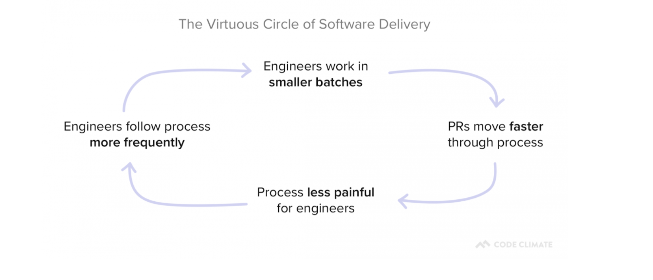
In addition, as you remove roadblocks from your development process, you’ll also reduce sources of frustration for your developers. This can have a positive impact on developer happiness and will set in motion a Virtuous Circle of Software Delivery, in which developers reap the benefits of optimization and are motivated to find even more ways to improve.

What’s Next?

Hopefully, you now have a better understanding of what Cycle Time is and why it matters. As a next step, you’re probably starting to think about ways to effectively minimize Cycle Time.

We took a data-driven approach to this question and analyzed thousands of pull requests across hundreds of teams. The results were interesting.

We turned that data into a tactical resource, The Engineering Leader’s Guide to Cycle Time, which offers a research-backed approach to minimizing Cycle Time.

If you’re interested in learning more about the origins of Cycle Time in Software Engineering, Mary and Tom Poppendieck’s book Lean Software, Chapter 4 “Deliver as Fast as Possible” is a great starting point.

If you would like to start tracking your own Code Cycle Time, request a consultation.

Related Resources

• What Data Science Tells Us About Shipping Faster
• The Engineering Leader’s Guide to Cycle Time
• Round Table: Perspectives on Cycle Time

Cycle Time in Lean Manufacturing

• “Takt Time – Cycle Time” – Describes some fundamental misconceptions around these terms. (Fittingly, the post includes a now 8-year running comment thread.)
• “How to Measure Cycle Times – Part 1”
• “How to Measure Cycle Times – Part 2”

Cycle Time in Software Engineering

• Lead time versus Cycle Time – Untangling the confusion
• The difference between Cycle Time and Lead Time… and why not to use Cycle Time in Kanban
• Measuring Process Improvements – Cycle Time?

Related Terminology

• Takt Time
• Lead Time
• Wait Time
• Move Time
• Process Time
• Little’s Law
• Throughput
• WIP

1 Thank you to Accelerate: Building and Scaling High Performing Technology Organizations, by Nicole Forsgren, Jez Humble and Gene Kim for the Donald Reinertsen reference, as well as the articulation of software development as having two primary phases (Chapter 2, p. 14 “Measuring Software Delivery Performance”). Accelerate is an excellent resource for understanding the statistical drivers behind software engineering. We were proud to have Nicole Forsgren speak at our Second Annual Code Climate Summit.

We last looked at Cycle Time for software engineering to understand what it is and why it matters. Most discussions about Cycle Time end there, leaving a lot of engineering managers frustrated and wanting more. Well-meaning and intelligent engineering managers have theories on which principles drive low cycle time, but very few actually have data to support their hypotheses.

So today we’re going to do just that – we’re going to reveal what we learned about cycle time after analyzing thousands of pull requests from hundreds of teams. In a field full of complexity and nuance, our analysis results were strikingly simple. The primary conclusion we came to was that there’s a single intuitive practice that is highly correlated with low cycle time. But it’s not the one we would have guessed.

The Data

Before we get into exactly our findings, let’s talk briefly about the dataset and definitions we used.

As a refresher, Code Cycle Time (a subset of Cycle Time) represents how long code remains “in flight” – written but not yet deployed.

Our data science team analyzed 180,000 anonymized pull requests from 500 teams, representing about 3,600 contributors. We asked the team to determine what correlation exists, if any, between the following software engineering delivery metrics (we called these “drivers”) and Code Cycle Time:

1. Time to Open (Days) (from commit to open)
2. Time to Review (Days) (from open to review)
3. PR Open to Merge (Days)
4. Number of Review Cycles
5. % of Abandoned Pull Requests
6. Pushes per Day
7. Pull Request Throughput per Week

While beyond the scope of this post, they used Locally Weighted Generalized Linear Models (GLM) to determine correlations between drivers.

The Results

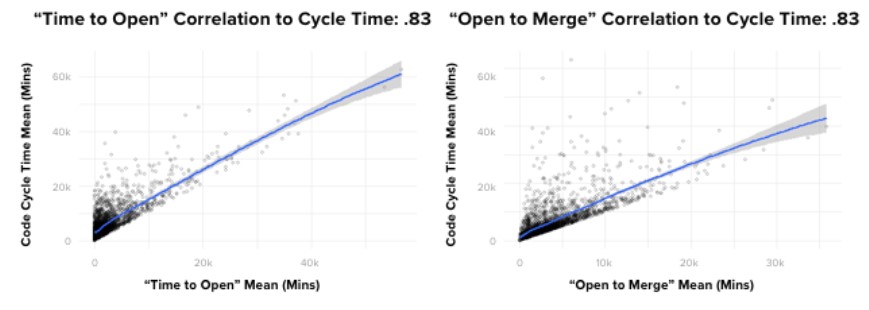
If I had been asked beforehand which of our set of metrics would prove most correlated with cycle time, I would have said, without hesitation, “PR Open to Merge”. Indeed, there is a powerful correlation between these two metrics. However, contrary to what you might think, the data showed that it’s not the most impactful one. Actually, of the drivers we looked at, the metric with the most predictive power on Code Cycle Time was, convincingly, Time to Open.

To give you a better sense of how strong the correlation is, in absolute terms, where a 0 coefficient means “no correlation” and 1 is perfectly correlated, Time to Open and Code Cycle Time had a 0.87 coefficient. This was, in fact, the strongest correlation we found between any two metrics we looked at in our analyses.

Even more striking, Time to Open is more predictive of Code Cycle Time than the length of time the pull request remains open, which means that pull requests that open faster, merge faster.

What can we do with this information?

First, as with most data-driven insights, it can be helpful to marry the results with our intuition.

Code that spends less time on someone’s laptop …

• Is likely small and therefore easier to get reviewed quickly by a single reviewer
• Gets reviewed sooner
• Gets closed sooner if it’s headed in the wrong direction (it happens)
• Signals to other team members the area of the codebase you are working, which can serve to head off painful merge conflicts before they happen

The good news is that Time to Open is a bit easier to influence and understand than the rest of Code Cycle Time, which can get mired in the complexity of collaboration.

Your team probably already hears from you about writing small pull requests, but reinforcing the message helps, and sharing data like the data presented here can help provide transparency and credibility to the recommendation.

One could also consider, carefully and judiciously, whether or not pair programming, in some cases, might improve time to open. This can be particularly helpful for engineers with a tendency (self aware or not) to overthink, overbuild and/or prematurely optimize code.

Closing

The influence of Time to Open on Code Cycle Time is striking. As software engineering professionals, we spend a lot of time discussing ways to optimize and understand the collaborative aspects of software development. This is completely understandable, and does in fact pay dividends. However, the data tells us that in some cases, for some teams, what you should be more likely looking at is your time to open.

Related Resources

• What is Cycle Time and Why Does it Matter?

Today, we’ll look at three terminal Pull Request outcomes and one way to improve abandoned Pull Requests and increase velocity in your engineering process.

Every Pull Request (PR) has one of three outcomes

Every PR has costs: engineering labor, product management, and opportunity cost, to name a few. Each also has an outcome: merged, closed without merging, or abandoned due to inactivity.

Here’s a look at how PRs fare across the industry:

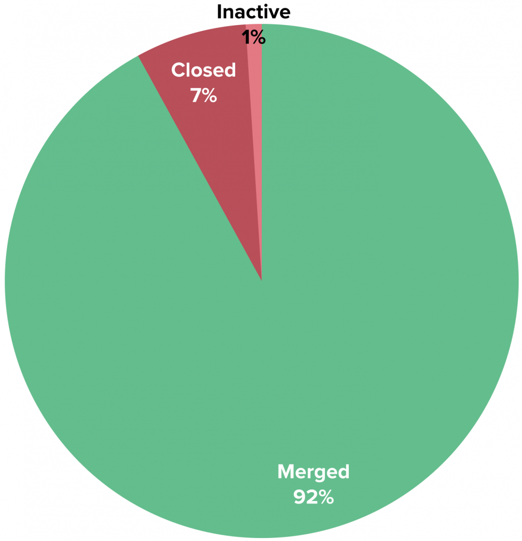
If you group closed and inactive Pull Requests together (“Abandoned PRs”), you can estimate that the average engineer abandons 8% of the Pull Requests they create, which is equivalent to a loss of $24,000 per year¹, or the cost of a 2018 Toyota Camry Hybrid.

We consider PRs that have had zero activity for more than three days to be abandoned because our data shows a very low likelihood that PRs that go untouched for so long get merged later.

Achieving zero abandoned Pull Requests is an anti-goal, as it would require being extremely conservative when opening them. However, a high rate of abandoned PRs can indicate inefficiency and opportunity for improvement within an engineering process. Reducing PR loss by 20% on a team with 10 engineers could save $48,000 per year.

How does my team stack up?

Using an anonymized, aggregated analysis of thousands of engineering contributors, we’re able to get an understanding of how an engineering organization compares to others in the industry:

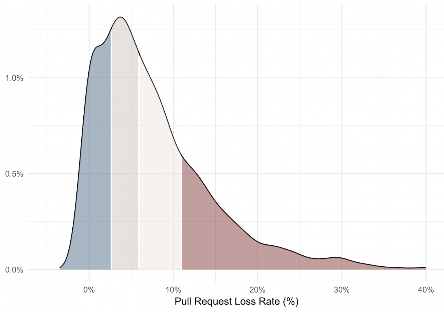
This density plot shows that the average Pull Request loss rate across our dataset is 8% (with a median of 6%). A loss rate above 11% would be in the bottom quartile, and a loss rate below 3% would be upper quartile performance.

Improving Pull Request outcomes

Abandoned Pull Requests are, of course, a lagging indicator. You can tell because it would be ridiculous to go to an engineering team and say, “All those PRs that you’re closing… merge them instead!”

Potential drivers lie upstream: late changing product requirements, shifting business priorities, unclear architectural direction and good ole’ fashioned technical debt. If you have an issue with abandoned Pull Requests, soliciting qualitative feedback is a great next step. Talk to your team. Identify something that is impacting them and talk about how you might avoid it next time. Then, rather than focus on the absolute value of your starting point, you can monitor that your abandonment rate is going down over time.

After all, you’d probably rather not send a brand new Camry to the scrap yard every year.

¹ Assumes a fully loaded annual cost of $300k per developer.

Learn how a Code Climate's Software Engineering Intelligence solution can offer visibility into engineering processes and improve your team's PR outcomes. Request a consultation.

Data-driven insights to boost your engineering capacity

Today we’re sharing something big: Code Climate Velocity, our first new product since 2011, is launching in open beta.

Velocity helps organizations increase their engineering capacity by identifying bottlenecks, improving day-to-day developer experience, and coaching teams with data-driven insights, not just anecdotes.

Velocity helps you answer questions like:

• Which pull requests are high risk and why? (Find out right away, not days later.)
• How does my team’s KPIs compare to industry averages? Where’s our biggest opportunity to improve?
• Are our engineering process changes making a difference? (Looking at both quantity and quality of output.)
• Where do our developers get held up? Do they spend more time waiting on code review or CI results?

Learn more about Velocity.

Why launch a new product?

Velocity goes hand-in-hand with our code quality product to help us deliver on our ultimate mission: Superpowers for Engineering Teams. One of our early users noted:

““With Velocity, I’m able to take engineering conversations that previously hinged on gut feel and enrich them with concrete and quantifiable evidence. Now, when decisions are made, we can track their impact on the team based on agreed upon metrics.” – Andrew Fader, VP Engineering, Publicis

Get started today

We’d love to help you level up your engineering organization. Request a demo here.

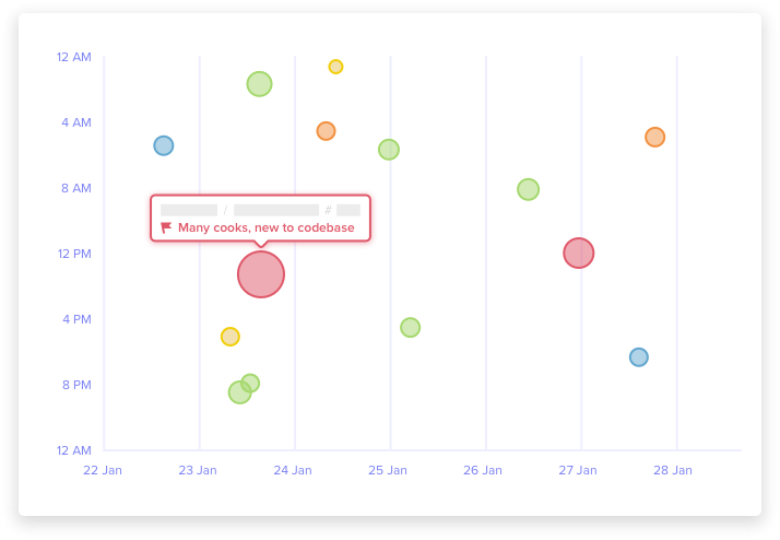
In the six years since we first introduced radically simple metrics for code quality, we’ve found that clear, actionable metrics leads to better code and more productive teams. To further that, we recently revamped the way we measure and track quality to provide a new, clearer way to understand your projects.

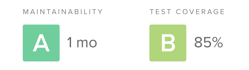
Our new rating system is built on two pillars: maintainability (the opposite of technical debt) and test coverage. For test coverage, the calculations are simple. We take the covered lines of code compared to the total “coverable” lines of code as a percentage, and map it to a letter grade from A to F.

Technical debt, on the other hand, can be a challenge to measure. Static analysis can examine a codebase for potential structural issues, but different tools tend to focus on different (and often overlapping) problems. There has never been a single standard, and so we set out to create one.

Our goals for a standardized technical debt assessment were:

• Cross-language applicability – A good standard should not feel strained when applied to a variety of languages, from Java to Python to JavaScript. Polyglot systems are the new normal and engineers and organizations today tend to work in an increasing number of programming languages. While most languages are based on primitive concepts like sequence, selection, and iteration, different paradigms for organizing code like functional programming and OOP are common. Fortunately, most programming languages break down into similar primitives (e.g. files, functions, conditionals).
• Easy to understand – Ultimately the goal of assessing technical debt with static analysis is to empower engineers to make better decisions. Therefore, the value of an assessment is proportional to the ease with which an engineer can make use of the data. While sophisticated algorithms may provide a seemingly appealing “precision”, we’ve found in our years of helping teams improve their code quality that simple, actionable metrics have a higher impact.
• Customizable – Naturally, different engineers and teams have differing preferences for how they structure and organize their code. A good technical debt assessment should allow them to tune the algorithms to support those preferences, without having to start from scratch. The algorithms remain the same but the thresholds can be adjusted.
• DRY (Don’t Repeat Yourself) – Certain static analysis checks produce highly correlated results. For example, the cyclomatic complexity of a function is heavily influenced by nested conditional logic. We sought to avoid a system of checks where a violation of one check was likely to be regularly accompanied by the violation of another. A single issue is all that’s needed to encourage the developer to take another look.
• Balanced (or opposing) – Tracking metrics that encourage only one behavior can create an undesirable overcorrection (sometimes thought of as “gaming the metric”). If all we looked for was the presence of copy and pasted code, it could encourage engineers to create unwanted complexity in the form of clever tricks to avoid repeating even simple structures. By pairing an opposing metric (like a check for complexity), the challenge increases to creating an elegant solution that meets standard for both DRYness and simplicity.

Ten technical debt checks

With these goals in mind, we ended up with ten technical debt checks to assess the maintainability of a file (or, when aggregated, an entire codebase):

1. Argument count – Methods or functions defined with a high number of arguments
2. Complex boolean logic – Boolean logic that may be hard to understand
3. File length – Excessive lines of code within a single file
4. Identical blocks of code – Duplicate code which is syntactically identical (but may be formatted differently)
5. Method count – Classes defined with a high number of functions or methods
6. Method length – Excessive lines of code within a single function or method
7. Nested control flow – Deeply nested control structures like if or case
8. Return statements – Functions or methods with a high number of return statements
9. Similar blocks of code – Duplicate code which is not identical but shares the same structure (e.g. variable names may differ)
10. Method complexity – Functions or methods that may be hard to understand

Check types

The ten checks break down into four main categories. Let’s take a look at each of them.

Size

Four of the checks simply look for the size or count of a unit within the codebase: method length, file length, argument count and method count. Method length and file length are simple enough. While these are the most basic form of static analysis (not even requiring parsing the code into an abstract syntax tree), most programmers will identify a number of times dealing with the sheer size of a unit of code has presented challenges. Refactoring a method that won’t fit all on one screen is a herculean task.

The argument count check is a bit different in that it tends to pick up data clumpsand primitive obsession. Often the solution is to introduce a new abstraction in the system to group together bits of data that tend to be flowing through the system together, imbuing the code with additional semantic meaning.

Control flow

The return statements and nested control flow checks are intended to help catch pieces of code that may be reasonably sized but are hard to follow. A compiler is able to handle these situations with ease, but when a human tasked with maintaining a piece of code is trying to evaluate control flow paths in their head, they are not so lucky.

Complexity

The complex boolean logic check looks for conditionals laced together with many operators, creating an exploding set of permutations that must be considered. The method complexity check is a bit of a hybrid. It applies the cognitive complexity algorithm which combines information about the size, control flow and complexity of a functional unit to attempt to estimate how difficult a unit of code would be to a human engineer to fully understand.

Copy/paste detection

Finally, the similar and identical blocks of code checks look for the especially nefarious case of copy and pasted code. This can be difficult to spot during code review, because the copied code will not show up in the diff, only the pasted portion. Fortunately, this is just the kind of analysis that computers are good at performing. Our copy/paste detection algorithms look for similarities between syntax tree structures and can even catch when a block of code was copied and then a variable was renamed within it.

Rating system

Once we’ve identified all of the violations (or issues) of technical debt within a block of code, we do a little more work to make the results as easy to understand as possible.

File ratings

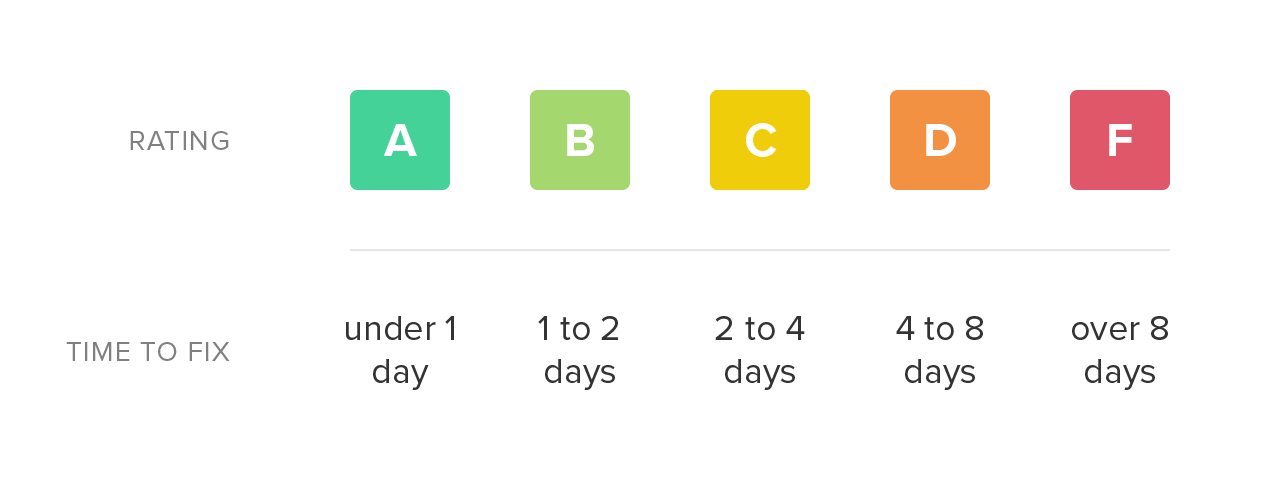
First, for each issue, we estimate the amount of time it may take an engineer to resolve the problem. We call this remediation time, and while it’s not very precise, it allows us to compare issues to one another and aggregate them together.

Once we have the total remediation time for a source code file, we simply map it onto a letter grade scale. Low remediation time is preferable and receives a higher rating. As the total remediation time of a file increases, it becomes a more daunting task to refactor and the rating declines accordingly.

Repository ratings

Last, we created a system for grading the technical debt of an entire project. In doing so, we’re cognizant of the fact that older, larger codebases naturally will contain a higher amount of technical debt in absolute terms compared to their smaller counterparts. Therefore, we estimate the total implementation time (in person-months) of a codebase, based on total lines of code (LOC) in the project, and compute a technical debt ratio: the total technical debt time divided by the total implementation time. This can be expressed as a percentage, with lower values being better.

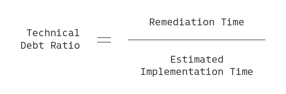
We finally map the technical debt ratio onto an A to F rating system, and presto, we can now compare the technical debt of projects against one another, giving us an early warning system when a project starts to go off course.

Get a free technical debt assessment for your own codebase

If you’re interested in trying out our 10-point technical debt assessments on your codebase, give Code Climate Quality a try. It’s always free for open source, and we have a 14-day free trial for use with private projects. In about five minutes, you’ll be able to see just how your codebase stacks up. We support JavaScript, Ruby, PHP, Python and Java.